Allusions to Shakespeare aside, the ability to inline functions, offered by modern languages such as C++, can deliver dramatic performance improvements while preserving proper design-semantics. However, the misuse or abuse of function inlining can also be highly detrimental to an application's performance, and while certain classes of function are obvious candidates for inlining, others are not. Moreover, inlining a given set of functions can affect performance in unexpected ways and while profiling tools are very useful, it does not follow that they are the Oracle of Delphi. To compound this, using a profiler is a post-compilation step, which runs contrary to pushing as much of the development process out of compile and run-time into design-time. This article therefore presents a way of visualising the interplay between the different factors that are involved in making an inlining decision.

|

|
An abridged version of this article appeared in the Oct/Nov 2003 issue of Application Development Advisor magazine, and another version (also abridged) appeared in the May 2004 issue of Dr Dobbs Journal of Programming. |
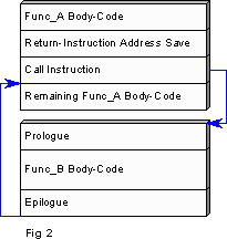
To recapitulate on the principles behind inlining, consider figure 1. This shows a simple function that does nothing except call another function, and in executing this call the CPU must perform certain essential housekeeping tasks. The details of these vary depending on processor design, but they include operations such as storing the address of the instruction to return to on completion of the call, and the saving of the caller's registers on the stack. Conversely, and before resuming execution of the caller, the CPU must perform the compliment of this housekeeping, which includes restoring the caller's register set, along with retrieving the address of the instruction to return to.
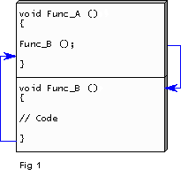
Given this, compilation of the code in figure 1 will yield machine-code sequences that look (in principle) like figure 2. The problem is that servicing these overheads delays the CPU, moreover, almost all function calls represent a branch in the instruction stream, which stall the CPU's pipeline, thus slowing execution still further as the pipe is refilled. Calculation of the branch-target address is also required.
To add to this the overhead code increases the size of the executable. This may be critical if primary storage is in short supply, and on multitasking platforms, larger executables compete more for space than smaller ones, thus causing more page misses. These in turn cause many thousands of additional machine cycles to be consumed as the required page is loaded from secondary storage. The worst-case scenario is when the branch to a frequently called function straddles a page boundary, which can cause thrashing.
Size also impinges on performance in terms of caching. The CPU's instruction and data cache is a relatively small amount of relatively fast storage, which holds a program's most frequently used instructions and data. Overhead code is cached just as much as the instructions that constitute the body of a function, thereby consuming space that could otherwise be occupied by other function bodies. If the processor cannot retrieve a function's instruction and/or data from the cache (a cache miss) then it must venture out onto the main bus to retrieve it from primary storage. Main-memory accesses are much slower than reading from the cache, plus they cause contention with other devices that wish to use the bus; this is something that we wish to avoid.
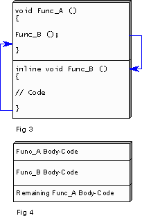
Now consider an alternative scenario depicted in figure 3. The situation is exactly the same as before except for the inclusion of the inline keyword in the source code. The change, however, in the compiled code is profound, as figure 4 demonstrates. The housekeeping has been eliminated, along with the call instruction, and the instructions representing the body of Func_B have been integrated into the body of Func_A.
As a result the code that constitutes the body of the function will execute faster, plus there is no longer a branch in the instruction stream, meaning that the pipeline continues to operate at peak efficiency. Further to this, the executable is smaller, meaning that it competes less with other applications for space and therefore causes fewer page misses; the problem of a call straddling a page boundary is also precluded. Moreover, the CPU's cache is put to better use because it now has more space for other data and instruction-sequences, which results in fewer cache misses and, from that, faster execution.
Straightforward as it may seem this is not a mandate for inlining everything and, compilation dependencies aside, three principal factors impinge on the decision to inline or 'outline' a given function. These are:
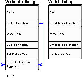
These factors interact in the following way: where the function is very small (say a simple accessor) the proportion of overhead costs to body or 'real' costs (OC:RC) is very large. Inlining such a function will improve performance as demonstrated earlier, and importantly, this is irrespective of the number of locations the function is called from. Moreover, the executable will shrink slightly. Figure 5 illustrates these points.
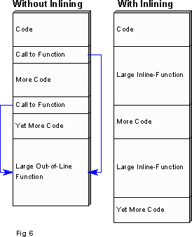
However, with larger functions the proportion of overhead to body code tends to the very small. Given that inlining, in principle, replicates the function body at each call site, many call sites will bloat the executable and reintroduce our caching and paging concerns. This could easily result in an executable that is slower than if we had not inlined at all. Figure 6 demonstrates these points.
Generally, therefore, the benefits of inlining larger functions are only retained if they are called from only one location. However, this size/static-frequency differential can be offset by how often a function is called in a typical run of the program. The more calls there are the more the overhead free benefit of inlining may be felt. Runtime popularity may therefore justify inlining a relatively large, statically frequent function, and here lies the challenge: Given the above arguments, can we construct a numerical model that better resolves the boundary between favourable and unfavourable inlining candidates?
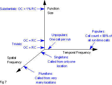
Firstly, it is clear that we are operating within a three-dimensional space, meaning that function size can be depicted graphically, along with spatial and temporal frequency. Secondly, while a given function's profile is highly platform dependent, if we quantify all three variables as proportions we can locate any function within the space. Consider figure 7.
The Function-Size axis represents the ratio of the overhead at a call site to the size of the outlined function body, in both space as well as time. This axis corresponds, at its lower limit, to empty global functions that take no parameters and return nothing. These are 'Trivials' where the proportion of real to overhead costs is very small (Minnows, to use a piscine analogy). There is, however, no theoretical upper-limit to function size, therefore the top end of the axis must be assumed to extend into the realm of functions with many thousands of lines of code, where the proportion of real to overhead is very large indeed — 'Substantials', to extend the terminology (or Whale Sharks; the biggest fish in the sea).
The Spatial-Frequency axis corresponds, at its lower limit, to a single call site in the executable (the realm of Singletons). Conversely, the upper limit can be assumed to correspond to a situation where 99.9% of function calls are calls to the inlining candidate ('Pluraltons', to develop the nomenclature further). Similarly, the Temporal-Frequency axis corresponds, at its lower limit, to a single execution of the inlining candidate during a typical run of the program (an 'Unpopular'), and at the upper limit to a situation where the CPU spends 99.9% of its time within the function in question.
Given this framework we can determine the spatial benefit of inlining a function as follows (we will examine the temporal side shortly): returning to first principles, we are trying to determine whether the function call-overhead is paying its way or proving to be dead weight. It follows that subtracting the cost of inlining from the cost of outlining will yield the overall saving that results if the function is inlined — its inlining 'favourability'. A negative result will mean that the cost of inlining exceeds that of outlining, meaning that the function should remain out of line. Expressed symbolically:
Spatial Inlining Favourability = Spatial Outlining Cost - Spatial Inlining Cost
Given that to inline means, in principle, to replicate the function body at each call site, the spatial inlining cost is equivalent to multiplying the function's size by its spatial frequency. I.e.:
Spatial Inlining Cost = Function Size * Spatial Frequency
Conversely, to outline a function means to replicate the call overhead at each call site. Given this, we can calculate the spatial outlining cost by subtracting function size from 1, and then multiplying the result by the spatial frequency. I.e.:
Spatial Outlining Cost = (1 - Function Size) * Spatial Frequency
Both of these terms scale the cost of inlining and outlining respectively. This reflects the costs of inlining or outlining in relation to a function's spatial frequency, and given these, the spatial cost/saving of inlining a function can be calculated as follows:
Spatial Inlining Favourability = (1 - Function Size) * Spatial Frequency
                               -      Function Size  * Spatial Frequency
Or, more formally, where F, s and fs denote Favourability, Size and Spatial Frequency respectively:
F = (1 - s)fs - sfs
Putting some real numbers into this yields the distribution shown in figure 8. [Note that a logarithmic scale is used in order to avoid filling the lower half of the table with positive (and therefore 'uninteresting') numbers — see the endnotes for a detailed explanation of this.] As theory demands, inlining functions of any size yields no appreciable saving when they are spatially infrequent. But, for very small functions, the saving increases dramatically as the proportion of calls increases. However, inlining functions that are a 50:50 mix of overhead and real execution costs yields no overall benefit, regardless of spatial frequency, and functions that have proportionally less and less overhead cost more and more if inlined.
| Function Size | Spatial Frequency | |||||||||||
| 0.00 | 0.00 | 0.50 | 0.75 | 0.87 | 0.94 | 0.97 | 0.98 | 0.99 | 0.99 | 1.00 | ||
| 0.99 | 0.00 | -0.50 | -0.75 | -0.87 | -0.93 | -0.97 | -0.98 | -0.99 | -0.99 | -0.99 | ||
| 0.99 | 0.00 | -0.50 | -0.74 | -0.87 | -0.93 | -0.96 | -0.98 | -0.98 | -0.99 | -0.99 | ||
| 0.99 | 0.00 | -0.49 | -0.74 | -0.86 | -0.92 | -0.95 | -0.97 | -0.98 | -0.98 | -0.98 | ||
| 0.98 | 0.00 | -0.48 | -0.73 | -0.85 | -0.91 | -0.94 | -0.95 | -0.96 | -0.97 | -0.97 | ||
| 0.96 | 0.00 | -0.47 | -0.70 | -0.82 | -0.88 | -0.91 | -0.92 | -0.93 | -0.93 | -0.94 | ||
| 0.93 | 0.00 | -0.44 | -0.66 | -0.77 | -0.82 | -0.85 | -0.86 | -0.87 | -0.87 | -0.87 | ||
| 0.87 | 0.00 | -0.38 | -0.56 | -0.66 | -0.70 | -0.73 | -0.74 | -0.74 | -0.75 | -0.75 | ||
| 0.75 | 0.00 | -0.25 | -0.38 | -0.44 | -0.47 | -0.48 | -0.49 | -0.50 | -0.50 | -0.50 | ||
| 0.50 | 0.00 | 0.00 | 0.00 | 0.00 | 0.00 | 0.00 | 0.00 | 0.00 | 0.00 | 0.00 | ||
| Fig. 8 | 0.00 | 0.50 | 0.75 | 0.87 | 0.93 | 0.96 | 0.98 | 0.99 | 0.99 | 0.99 | ||
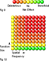
This distribution can be mapped into a colour space (by dividing F by 4) as indicated in figure 9. Red means that the function should not be inlined, yellow means that the merits and demerits of inlining a given function cancel each other out, and green indicates that inlining will be beneficial.
Using this scheme the table can be rendered as shown in figure 10.
So far so good, but this only tells us what we already knew. The object of the exercise is to see how temporal frequency offsets matters; therefore we must include that factor in the equation too.
Returning again to first principles, an outlined call entails an overhead in time as well as space, and the more often the call is made the more often that price is paid. From this, and in the same fashion as calculating the spatial overhead, the temporal cost of outlining can be determined by subtracting the real cost of the function from 1 and multiplying that by the temporal frequency, or:
Temporal Outlining Cost = (1 - Function Size) * Temporal Frequency
Now, previously we balanced the spatial costs of inlining against those of outlining, but in the temporal case we only pay if a function is out of line — by definition, to inline is (in principle) to lose the time overhead. Given this, we need incorporate the temporal factor only once into the equation, which would suggest the following:
Favourability = Spatial Outlining Cost + Temporal Outlining Cost
              - Spatial Inlining  Cost
However, we are working with proportions and cannot simply add the two outlining costs together because this would give an incorrect result. The correct way is to take the sum and then subtract the product.[See the endnotes for the logic behind this] That is to say:
Total Outlining Cost = Spatial Outlining Cost + Temporal Outlining Cost
                     - Spatial Outlining Cost * Temporal Outlining Cost
Given this, the inlining favourability of a function can be expressed in the following way:
Favourability = Spatial Outlining Cost + Temporal Outlining Cost
              - Spatial Outlining Cost * Temporal Outlining Cost
              - Spatial Inlining  Cost
Formally, therefore, the favourability of inlining a given function can be calculated as follows, where ft denotes Temporal Frequency:
F = (1 - s) * fs + (1 - s) * ft
  - (1 - s) * fs * (1 - s) * ft
  - sfs
Which can be simplified to yield:
F = (1 - s)fs + (1 - s)ft - fsft(1 - s)2 - sfs
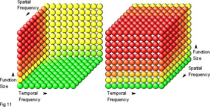
Using real numbers with this equation, and the same colour scheme as before, we can render a three-dimensional 'inlining-decision space', and this is shown in figure 11.
What is immediately apparent is that the space is skewed towards choosing not to inline. Mostly it is coloured red, orange and yellow because it is a situation of two against one — plurality and size, against popularity, which translates to the risk of executable bloat against our wish to hurry the processor along.
In the best-case scenario, at the lower front-right of the space, it is those popular little minnows, which are called everywhere that make a real difference when inlined. Conversely, those temporally unpopular, spatially frequent Whale Sharks, which lie at the top front-left of the space should remain forever out of line. Not, it should be said, that such behemoths should ever arise in any self-respecting developer's code. They indicate a poor understanding of design, coding and compilation issues, one in which the issue of inlining is superfluous.
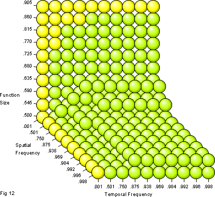
Now that we have a full distribution, the unfavourable part can be excised to leave just the area where inlining is beneficial. By adopting a linear rather than logarithmic scale for function size, and then concentrating only on the 0.500 to 0.905 range (for that axis) it is possible to zoom in on the boundary and thus answer the original question.
This is shown in figure 12 and demonstrates, for example, that temporally popular Singletons have an upper limit (in this model) of 0.86 in terms of real costs to overhead costs, past that it is not worth inlining them.
There are, however, many additional elements that should be included in the equation. As it is, the model considers outlining costs at the call-site because these are paid, spatially, at every call site, and paid temporally every time the function is invoked. However, it does not consider the costs of the prologue/epilogue within the outlined function. In the spatial case, this is not a significant problem as this cost is incurred only once, at the function's location within the executable, and would not offset the above results noticeably. However, with the temporal axis, this cost really should be included because every run-time invocation incurs a temporal overhead at both the call site and in the execution of the prologue/epilogue code.
Given this, the function-cost proportion can be split into separate temporal and spatial components, which are then scaled by their respective frequencies. Expressed symbolically:
Favourability = Spatial  Outlining Cost * Spatial  Frequency
              + Temporal Outlining Cost * Temporal Frequency
              - Spatial  Outlining Cost * Spatial  Frequency
              * Temporal Outlining Cost * Temporal Frequency
              - Spatial  Inlining  Cost * Spatial  Frequency
Which, formally, translates to the following, where ss and st represent the function's 'size' in space and time respectively:
F = (1 - ss)fs + (1 - st)ft - (1 - ss)fs(1 - st)ft - ssfs
Sadly, however, this robs us of a convenient graphical depiction of the decision space, as it is not possible (reasonably) to render a four dimensional space in two dimensions. Although we could use a workaround, and depict a set of decision spaces, ranged along, say, the temporal axis.
However, graphics aside, and despite its increased accuracy, this refined model is still far from complete, in that we have yet to consider the nature of the function in question. Semantically, one block of source code can differ radically to another, and this can have a great bearing on the decision to inline. For example, functions range from being entirely compute-bound to being entirely I/O bound, and by definition, I/O-bound functions use the system bus more frequently than compute-bound ones. This makes them poorer candidates for inlining, whereas compute-bound functions hold more of their data in registers (the fastest form of storage), making them very good candidates for inlining.
Extending the question of a function's nature, we should consider the impact of inlining on optimisation. A compiler can implement a given function in a variety of ways, while preserving semantic equivalence. Some ways yield code that is smaller and/or faster, and to choose this end of the spectrum is to optimise for size or performance respectively. In fact, optimisation can be viewed as a form of compiler-determined refactoring, and the degree to which a compiler can optimise a given function depends in part on how much it knows about that function. This is why C++ language-features such as const are so valuable; they provide design-time guarantees to the developer, while providing compile-time guarantees to the compiler.
Now, while inlining is a powerful optimisation in itself (when used correctly), a call to an inline function renders the function body visible from within the caller. Given that this means a better-informed compiler, this makes additional, powerful, optimisations available. Consider a function that calls another from within a loop, where the second function is a trivial accessor. If the compiler knows that the number of iterations is constant it can unroll the loop, but may choose not to because there are just a few too many iterations, given the overhead of calling the function. Yet if the accessor is inlined then the compiler now knows that it does nothing except return a value. In this case it would be much more likely to perform loop unrolling because it can elide the second function's code, such that it ceases to exist at the machine level.
Using the same principles as before, we can therefore symbolise a function's inlining favourability, in terms of its compute binding and optimisation potential (once again observing the rule of adding proportions):
Favourability = Compute Binding + Optimisation Potential
              - Compute Binding * Optimisation Potential
We can then subtract this from 1, and use the result to scale the spatial-inlining cost, such that a high Compute-Binding/Optimisation-Potential reduces it, thus making inlining more attractive. The main equation can therefore be extended further to give:
Favourability = Spatial  Outlining Cost * Spatial  Frequency
              + Temporal Outlining Cost * Temporal Frequency
              - Spatial  Outlining Cost * Spatial  Frequency
              * Temporal Outlining Cost * Temporal Frequency
              - Spatial  Inlining  Cost * Spatial  Frequency
              * (1 - (Compute Binding + Optimisation Potential
              -       Compute Binding * Optimisation Potential))
Or, formally, where c and o denote compute binding and optimisation potential respectively:
F = (1 - ss)fs + (1 - st)ft - (1 - ss)fs(1 - st)ft - ssfs
  * (1 - (c + o - co))
At this point, however, we are wading into some very deep water. Locating an actual function in the decision space 'by hand' is possible if one can provide precise numbers for size and temporal frequency. However, ascertaining a function's degree of compute binding is more challenging, and determining a function's potential for optimisation is quite another matter, which depends on the most intimate knowledge of one's compiler, as well as a fair-old understanding of the language. Ultimately, the metric that we calculate might bear no relation to reality. Moreover, if an inline function contains other inline calls (and so on, recursively) then calculating its favourability metric is redundant because the code that is generated could be very distant indeed from the code that we wrote originally.
Then there is the target platform to consider. Processors with larger register files will suffer less from register spill, meaning that less of a function's data need be placed on the stack, which in turn improves performance. Similarly, systems with larger caches will suffer less from cache misses, and (continuing down the storage hierarchy), platforms with larger amounts of primary storage will suffer less from page misses. On the temporal side of things, a CPU that can perform speculative execution will suffer less from stalled pipelines, which in turn ameliorates the problem of branches in the instruction stream. All of these factors impinge on the favourability of inlining a given function, and while they should therefore be factored into the model, providing precise figures for the various factors is virtually impossible.
However, with compilers it is, or could be, a different matter. In principle, a compiler can provide accurate estimates for most of the above factors, up to and including issues relating to the target CPU's architecture. (Although we would still need a profiler to measure temporal frequency, as even a compiler cannot predict future runs of a system.) In reality, however, current compilers only 'see' one translation unit at a time, rather than the totality of a system's code, meaning that they cannot generate a global view of a system. Given this, they will be unable to automate the inlining decision-process completely unless we abandon the per-file compilation model in favour of 'global' compilation. Until then, developers will have to address the fascinating intricacies of inlining themselves.
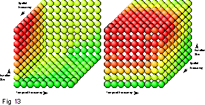
Finally, and aside from the true complexities of this issue, seasoned developers may opine that they already understand the various tradeoffs intuitively. However, here lies an important lesson. This treatise began life as an informal handout for a group of developers who attended a high-performance C++ training course. As a somewhat rough and ready illustration of inlining criteria the decision space presented included the basic temporal and spatial factors that we started with, but was, in part, an educated guess. This is shown in figure 13, and to compare it with the one in figure 11, which was generated numerically, is revealing. Specifically, I overestimated the degree to which a high temporal-frequency compensates for a high spatial-frequency with larger functions. Clearly, the numbers do not support my sunny optimism, and the upshot is that, while intuition gets us most of the way, to be absolutely sure you must go to hard data.
For further explanation and exploration of the issues pertaining, specifically, to inlining and to performance-oriented C++ in general, Efficient C++ by Bulka and Mayhew is an excellent starting point. Note, however, that while the authors discuss static call-frequency as a criterion, the inlining-decision matrix[Bulka & Mayhew 135] that they present only plots function size against temporal frequency, and is not founded on a numerical model.
Efficient C++ — Performance Programming Techniques
Bulka and Mayhew
Addison Wesley
ISBN 0 201 37950 3
A delegate on a high-performance programming course asked why I chose a non-linear scale in the depiction of the full inlining-decision space (although the diagram that zooms in on the precise cost/benefit threshold does use a linear scale).
The reason for this, and to reiterate the arguments presented above, is that inlining everything that falls below the 50% mark on a linear scale (in terms of the proportion of function body-code to overhead code) will always be favourable. This is because one is always replacing the call overhead with the (smaller) function body, meaning the executable will always be smaller. This in itself will always improve performance, by however small an amount, and is an auxiliary speed-up to that which comes from eliding the temporal call-overhead.
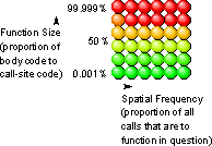
Given this, everything in the lower half of a linearly-scaled space will be green, and it struck me that there was no point in taking up so much of the diagram with what we already know. The diagram illustrates this, and is a mini, linear, (and intuitive) version of Fig 10.
Ultimately, therefore, I chose a non-linear scale in order to emphasise the area of uncertainty, while still depicting the whole space — it's just the way that I approached it at the time.
I also received an email from a DDJ reader asking why one must take the sum and subtract the product when working with proportions. I didn't go into this above because I didn't want to get off-topic, but in essence the problem is that simply adding the terms does not give the correct answer. For example, if you add two proportions that are greater than 0.5, you get a result that is greater than 1. This may be just what you want in other situations, but the inlining model is based entirely on a proportional model, and a proportion must, by definition, be between 0 and 1. Given this, the logic behind adding one proportion to another correctly is as follows:
If you have a proportion that is equal to 0.75, then subtracting that from 1 gives 0.25. To add another proportion you use the 0.25 to scale that factor down before doing the addition. In other words, when adding two proportions you take the first, and then add the second within the bit that's left over. Given this, the sum of two proportions can be expressed as follows:
Sum = p1 + (1 - p1) * p2
...Where the rules of operator precedence mandate that the operation in brackets is completed first, then the multiplication, followed by the addition. There is nothing wrong in expressing the equation in this way, but it can be refactored such that one first multiplies the two proportions, and then subtracts that from the figure yielded by adding them. In other words you take the sum of the two proportions and subtract the product, or:
p = p1 + p2 - p1 * p2
...Which is identical semantically to the first form, but has less brackets, and is therefore simpler. It is also the form used in statistics, where probabilities are expressed as proportions, and where one is faced with calculating the probability of, for example, an early death that arises from a high-fat diet combined with no exercise.
The important thing is that this scaling-down principle can be extended such that a third factor can be added in the same fashion. However, the following equation is not the correct method:
p = p1 + p2 + p3 - p1 * p2 * p3
This, as before, would give an incorrect result. In fact the correct extension of the principle is to take the result of the two-proportion addition, and then use that with the third factor to calculate a fresh sum and product. That is to say:
p = (p1 + p2 - p1 * p2) + p3 - (p1 + p2 - p1 * p2) * p3
...Which can be extended in the same way to take in a fourth, fifth, etc. factor. It also follows that the alternative form of this equation is:
p = p1 + (1 - p1) * p2 + (1 - p1 + (1 - p1) * p2) * p3
Which is more complicated because of the extra brackets.